Animation And Convex Hull In Bokeh
This blog post looks at creating an animation slider (with Play and Pause buttons) to plot 2D coordinates of player movement in a soccer game. Also, this post explains the steps to create a toggle button, to show/hide the convex hull plot of the teams. I’ve used Bokeh to plot the viz. Bokeh gives a good looking viz in the browser and also provides smooth interface for animation. I’ve also tried the same with Matplotlib and it was successful. But the features of bokeh (compared to matplotlib) makes it a better choice, for this purpose alone. I could write a separate blog post to outline the process in Matplotlib.
The dataset used in the post is from STATS. You can submit an online request to obtain the dataset from them. The data used in the viz is not available for public use.
Note that I’ve already done some pre-processing to clean the raw data since the data from STATS doesn’t have player/team tags and we’d have to manually add them. I’m not going to explain in depth about the data cleaning process. Once you get the dataset and have doubts on adding team/player tags, do contact me on twitter/mail. Also, an similar dataset can be used (for any sports) as long as you’ve the below columns.
Once you’ve the data file ready, create the below folder directory, which would be needed to run the bokeh server.
myapp
|
+—data (folder)
| +—data.csv
|
+—main.py
+—static (folder)
| +—images (folder within static)
| | +—pitch_image.png
Once the player and team tags are added, we’d have the data as below
    import pandas as pd
    df=pd.read_csv('data/data.csv')
    headers = ["x", "y", "team_id", "player_id","time"]
    all_team = pd.DataFrame(df, columns=headers)
Here, x and y: Player coordinates on the pitch, team_id: 1 and 2 for each team respectively, 3 for ball, player_id: Ranges from 1-11 for both teams, 12 for ball time: time of sequence.
Now import all necessary packages.
    # -*- coding: utf-8 -*-
    import numpy as np
    import pandas as pd
    from bokeh.io import curdoc
    from bokeh.layouts import row, widgetbox,column
    from bokeh.models import ColumnDataSource,LabelSet,PointDrawTool,CustomJS
    from bokeh.models.widgets import Slider,Paragraph,Button,CheckboxButtonGroup
    from bokeh.plotting import figure
    from scipy.spatial import ConvexHull
My game sequence time starts at 0. So I’ve created a variable to initialise time and calculated initial player coordinates based on that. Since my slider time will always start at 0 (when the plot is displayed on browser), I’ve initialised the time here as 0.
    i=0

    x = all_team[all_team.time==i].x  #Calculate x based on time
    y = all_team[all_team.time==i].y  #Calculate y based on time
To plot the player labels and team colour, I’ve created 2 separate variables player_id and c. This is bit like hard coding the labels and colour. Since these values will not change for the whole sequence, it doesn’t matter if we hard code this or use any other alternative method. You could also use factor_cmap feature on bokeh, for player color.
    player_id=['1','2','3','4','5','6','7','8','9','10','11','1','2','3','4','5','6','7','8','9','10','11',' ']

    #The last value is left empty to not show label for the ball.

    c=['dodgerblue','dodgerblue','dodgerblue','dodgerblue','dodgerblue','dodgerblue','dodgerblue','dodgerblue','dodgerblue','dodgerblue','dodgerblue','orangered','orangered','orangered','orangered','orangered','orangered','orangered','orangered','orangered','orangered','orangered','gold']
Once we’ve the required variables, create the ColumnDataSource as below.
source = ColumnDataSource(data=dict(x=x, y=y,player_id=player_id,color=c))
Now we should plot the background image (football pitch). For this, store the image inside the static/images folder within myapp folder.
Now create the plot as below.
    #Set up plot
    plot = figure(name='base',plot_height=600, plot_width=800, title="Game Animation",
                  tools="reset,save",
                  x_range=[-52.5,52.5], y_range=[-34, 34],toolbar_location="below")

    plot.image_url(url=["myapp/static/images/base.png"],x=-52.5,y=-34,w=105,h=68,anchor="bottom_left")
    #x,y,w,h are given based on STATS definition of the dataset
    #hide axis and grid lines
    plot.xgrid.grid_line_color = None
    plot.ygrid.grid_line_color = None
    plot.axis.visible=False


    #Plot the player coordinates
    st=plot.scatter('x','y', source=source,size=20,fill_color='color')

    #Add labels to the scatter plot
    labels=LabelSet(x='x', y='y', text='player_id', level='glyph',
                      x_offset=-5, y_offset=-7, source=source, render_mode='canvas',text_color='white',text_font_size="10pt")

    plot.add_layout(labels)

    layout = column(row(plot))  #add plot to layout

    curdoc().add_root(layout)

    curdoc().title = "Game Animation"
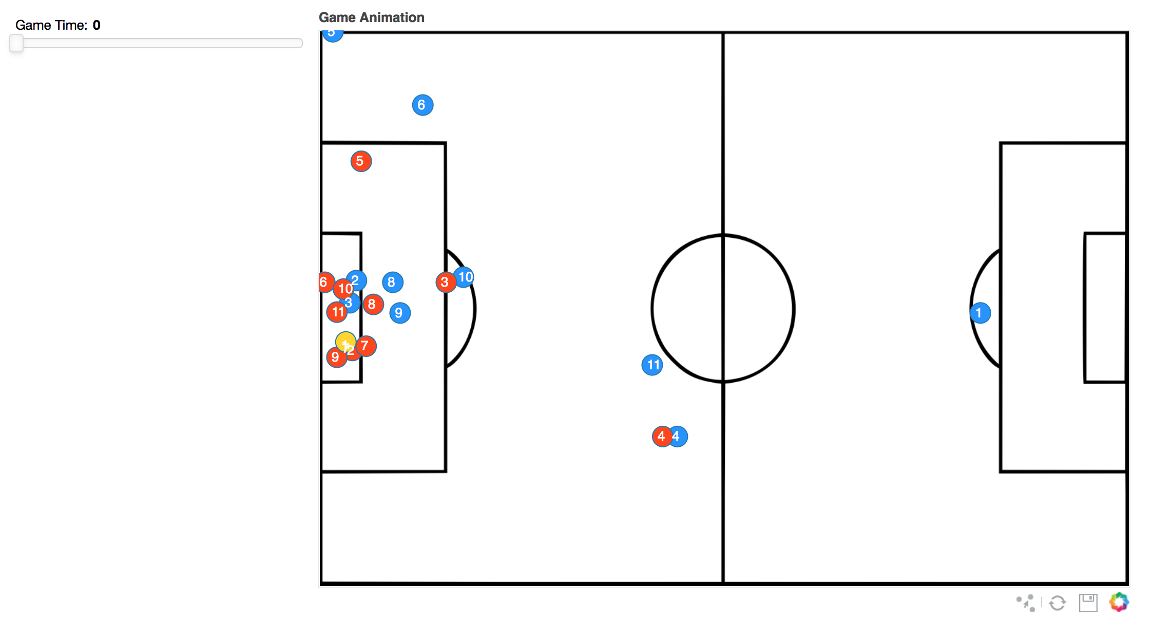
Now run the bokeh server using bokeh serve –show myapp. For the plot to appear, run the bokeh serve from the directory where your myapp folder is placed. For example, If the myapp folder is located inside your desktop/python directory, traverse (cd desktop/python) to the folder on terminal/cmd and run the bokeh serve command. This should show the plot in the browser.
The plot will only show the player coordinates at time 0. Now we need to add a slider and vary the time to show the full sequence of event.
    #Add a slider freq
    freq = Slider(title="Game Time", value=0, start=all_team.time.unique().min(), end=all_team.time.unique().max(), step=1)
We define the start and end time using all_team.time.unique().min()/max().
Once the slider is created, you’d need to build a function to get the call back when slider is updated.
    def update_data(attrname, old, new):
        k = freq.value #holds the current time value of slider after updating the slider

        #now again plot x and y based on time on slider
        x = all_team[all_team.time == k].x
        y = all_team[all_team.time == k].y
        #update the CDS source with new x and y values. player_id and c remains same and it'll be plotted on top of new x and y.

        source.data = dict(x=x, y=y,player_id=player_id,color=c)
Every time the source gets updated, all the plots associated with ‘source’ will get updated as well, which includes the scatter plot st and labels, since we’re using this source to plot those data.
To call the above function when the slider is updated, we add
    for w in [freq]:
        w.on_change('value', update_data)
Now add the slider to the plot layout using the Widgetbox.
inputs = widgetbox(freq)
Now if you run the bokeh serve again, you should be able to see the slider and the plot gets updated based on the change in the slider.
Now add the button to create the play and pause animation.
button = Button(label='► Play', width=60)
To allow ► symbol in your browser, add “# -- coding: utf-8 --” in the beginning of your code.
    def animate_update():
        year = freq.value + 1 #gets value of slider + 1
      if year > all_team.time.max():
            year = all_team.time[0]  #if slider value+1 is above max, reset to 0
        freq.value = year
    #Update the label on the button once the button is clicked
    def animate():
        if button.label == '► Play':
            button.label = '❚❚ Pause'
      curdoc().add_periodic_callback(animate_update, 50)  #50 is speed of animation
        else:
            button.label = '► Play'
      curdoc().remove_periodic_callback(animate_update)

    #callback when button is clicked.
    button.on_click(animate)
The animate button was taken from here: Gapminder Bokeh
Update the WidgetBox with the button and run the bokeh server to see the animation.
inputs = widgetbox(freq,button)
To plot the convex hull, we’d need to create few more variables.
    team_att =all_team[all_team.team_id==2]
    team_def =all_team[all_team.team_id==1]
We’ve now split the data frame to hold separate data for attacking and defending team, since we’d have to plot convex hull for each team.
We then use numpy’s vstack feature to create the 2 arrays.
    t1 = np.vstack((team_att[team_att.time==i].x, team_att[team_att.time==i].y)).T
    t2 = np.vstack((team_def[team_def.time == i].x, team_def[team_def.time == i].y)).T
Once we have the arrays, we use the scipy convex hull package to get the vertices of the convex hull.
    hull=ConvexHull(t1)
    hull2= ConvexHull(t2)
    xc = t1[hull.vertices, 0]
    yc = t1[hull.vertices, 1]

    ax = t2[hull2.vertices, 0]
    ay = t2[hull2.vertices, 1]
Create 2 separate CDS to hold these values.
    source2 = ColumnDataSource(data=dict(xc=xc,yc=yc))
    source3 = ColumnDataSource(data=dict(ax=ax,ay=ay))

    #Plot the vertices as a patch
    team_Blue=plot.patch('xc', 'yc', source=source2, alpha=0.3, line_width=3, fill_color='dodgerblue')
    team_red = plot.patch('ax', 'ay',source=source3, alpha=0.3, line_width=3,fill_color='orangered')
If you run the bokeh server now, the convex hull will be plotted only for the time 0 since we’ve not added source2 and source 3 in the slider call bck. In the function update_data, again add the above steps to plot the convex hull dynamically, based on the slider value.
Now, the updated function update_data looks as below:
    def update_data(attrname, old, new):

        k = freq.value

        x = all_team[all_team.time == k].x
        y = all_team[all_team.time == k].y
        source.data = dict(x=x, y=y,player_id=player_id,color=c)


        t1 = np.vstack((team_att[team_att.time==k].x, team_att[team_att.time==k].y)).T
        t2 = np.vstack((team_def[team_def.time==k].x, team_def[team_def.time==k].y)).T

        hull = ConvexHull(t1)
        hull2= ConvexHull(t2)
        xc = t1[hull.vertices, 0]
        yc = t1[hull.vertices, 1]

        ax = t2[hull2.vertices, 0]
        ay = t2[hull2.vertices, 1]


        source2.data=dict(xc=xc,yc=yc)
        source3.data=dict(ax=ax,ay=ay)
So now if you run the bokeh server, the convex hull also will be updated when the slider gets updated.
Now to toggle the convex hull on/off, add a CheckboxButtonGroup to the plot.
    checkbox_blue=CheckboxButtonGroup(labels=["Team Red"],button_type = "primary")
    checkbox_red=CheckboxButtonGroup(labels=["Team Blue"],button_type = "primary")
There are multiple ways to toggle the convex hull on/off. I’ve used the CustomJS option to set the convex hull patch alpha when the toggle button is clicked.
Update the plot.patch as below, so that the patch is initially not visible in the plot.
    #alpha is changed to 0
    team_Blue=plot.patch('xc', 'yc', source=source2, alpha=0, line_width=3, fill_color='orangered')
    team_red = plot.patch('ax', 'ay',source=source3, alpha=0, line_width=3,fill_color='dodgerblue')
Now add a customJS callback to these patches. This callback will update the patch alpha to 0.3. This is a shortcut to make this work. The other alternative solution would be to add the convex hull plot as a children to the plot layout.
    #l0.glyph.fill_alpha sets the alpha of the patch
    checkbox_blue.callback = CustomJS(args=dict(l0=team_Blue, checkbox=checkbox_blue), code="""
    l0.visible = 0 in checkbox.active;
    l0.glyph.fill_alpha = 0.3;
    """)
    checkbox_red.callback = CustomJS(args=dict(l0=team_red, checkbox=checkbox_red), code="""
    l0.visible = 0 in checkbox.active;
    l0.glyph.fill_alpha = 0.3;
    """)
Add a paragraph label and update the WidgetBox and run the server.
    p = Paragraph(text="""Select team  to plot convex hull""",
    width=200)

    inputs = widgetbox(freq,button,p,checkbox_blue,checkbox_red)
The completed output should be like this.
Since bokeh plots are easy to use, you can modify the plot based on your own preference.
Hope this post provide a clear explanation on the steps involved. In case you’ve questions, please find my contact details on the contact page.
The complete code can be found here.
I’d highly appreciate your comments and feedback regarding the post/code used here.
Thanks.